R programming
Part of Course: Data Science Bootcamp #12
Why R?
ภาษา R เป็นภาษาที่สร้างขึ้นเพื่อ Data Science โดยเฉพาะ เราเรียก R ว่า "Fast data crunching tool" ก็คือ ติดตั้งเสร็จ ทำงานกับ Data ได้เลย เพราะมัน Native Support อยู่แล้ว ที่สำคัญคือ ใช้ได้ฟรี
Tool ที่เกี่ยวข้อง
Postit.cloud (ชื่อเดิมคือ RStudio Cloud)
เขียนภาษา R ผ่าน Web Browser
Desktop
Base R
https://cran.r-project.org/bin/windows/base/
ตัว Support ภาษาบน Desktop
R Studio IDE
https://posit.co/download/rstudio-desktop
ถ้าใช้ตัวนี้ แนะนำให้เราเช็ค Working Directory ก่อน ถ้าต้องการเปลี่ยนให้คลิกเมนู Session > Set Working Directory > Choose Directly และเลือก / สร้างโฟลเดอร์ที่ต้องการ
หลังจากเลือกโฟลเดอร์ จะแสดง Console
> setwd("[path]")
คำสั่งที่ใช้เช็ค
> getwd()
Keyboard Shortcut (R Studio IDE)
Mod = Ctrl (Windows) / Cmd (Mac)
# Clear
Mod + L

# Reproduce
Highlight Code in script and press
Mod + Enter
Variables
name <- value / expression

หรือ

name = value / expression
ลบตัวแปร
rm(var)
Operator ที่ใช้ได้
>>=<<===(equal)!=(not equal)
Data Types
numeric- ตัวเลข เช่น10character- ตัวอักษร หรือข้อความ เช่น"Taylor"logical- Expression เช่น1 + 1 == 2มีค่าTRUE,FALSEพิมพ์ย่อT,Ffactor- ตัวแปร categorical ในทางสถิติ เป็นตัวสำคัญในการทำงาน เช่นfactor(c("Red", "Blue", "Green"))date- ข้อมูลวันที่
การตรวจสอบ type
class(var)
Logical
ต่าที่เป็น True
- ค่าที่ไม่ใช่ 0
- T
- TRUE
- "TRUE" (case-insensitive)
ค่าที่เป็น False
- 0
- F
- FALSE
- "FALSE" (case-insensitive)
Factor
เราสามารถสร้างชุดข้อมูลแบบนี้
colors <- c("Red", "Blue", "Green")
แต่เมื่อใช้ class ปรากฎว่ามันได้ผลเป็น Character
class(colors)
> "character"
เมื่อลอง print จะได้ผลดังนี้
print(colors)
> "Red" "Blue" "Green"
เราจะเปลี่ยนเป็น Factor ต้องครอบด้วย factor()
colors <- factor(colors)

## print
print(colors)
> Red Blue Green
Factor จะไม่มี "" ครอบ
Date
## เวลาปัจจุบัน
time_now <- sys.time()

class(time_now)
> "POSIXct" "POSIXt"
Convert Data Types
as.numeric()
as.character()
as.logical()
Data Structure
- Vector
- Matrix
- List
- DataFrame
Vector
## Vector เก็บชุดข้อมูลที่มี Data Types เดียวกัน
## colon
1:10
> 1 2 3 4 5 6 7 8 9 10

## function seq
seq(from = 1, to = 100, by = 5)
## จะนับค่า 1 ไป 100 โดยบวกทีละ 5

## function c
colors <- c("Red", "Blue", "Green")
ages <- c(30, 31, 25, 29, 32)
Matrix
v <- 1:25
dim(x) < - c(5, 5)
## ผลที่ได้ จะแบ่งข้อมูล vector เป็น 5x5

## matrix(data, ncol=?)
matrix(1:25, ncol=5)
## ได้ผลเหมือนกับข้างบน

## matrix(data, ncol=?, nrow=?)
matrix(1:6, nrow=3, ncol=2)
## ได้ผลเป็น
## 1 3 5
## 1 4 6

## ถ้าอยากเรียงตามแถว ให้เพิ่ม byrow=T
matrix(1:6, nrow=3, ncol=2, byrow=T)
## ได้ผลเป็น
## 1 2 3
## 4 5 6

## element wise computation
matrix_var  + 102
## 102 ถูกบวกทุก element
List
## list เก็บข้อมูลหลาย Data Type ได้
my_list <- list(
name = "Ice",
age = 30,
scores = c(90, 85, 88),
passed = TRUE
)

## print list ออกมา
my_list

## print item
my_list$scores
Data Frame
เป็น Data Structure ที่มีความสำคัญต่อการทำงานเป็น Data Analyst เป็นที่เก็บข้อมูล Structured Data ซึ่งเราใช้ทำงานมากกว่า 80%
## การสร้าง Data Frame
## Create from vector
customers <- c("Ann", "Bob', "Christina")

ages <- c(25, 30, 22)

locations <- c("Bangkok", "Chiang Mai", "Phuket")

cus <- data.frame(customers,
		          ages,
		          locations)
cus
## Result
##   customers    ages    locations
## 1       Ann      25      Bangkok
## 2       Bob      30   Chiang Mai
## 2 Christina      22       Phuket

## ตั้งชื่อคอลัมน์
cus <- data.frame(
	Name = customers,
	Age = ages,
	City = locations)
cus
## Result
##       Name     Age         City
## 1       Ann      25      Bangkok
## 2       Bob      30   Chiang Mai
## 3 Christina      22       Phuket

## View as graphical table
## v -- ใช้ V ตัวพิมพ์ใหญ่
View(cus)

## Create from list
my_list <- list(Name = customers, Age = ages, City = locations)

cus <- data.frame(my_list)
cus
## Result
##       Name     Age         City
## 1       Ann      25      Bangkok
## 2       Bob      30   Chiang Mai
## 3 Christina      22       Phuket
Subset
## -- By position
customers <- c("Ann", "Bob', "Christina")

customers[1]
## > "Ann"

customers[3]
## > "Christina"

customers[1:2]
## > "Ann" "Bob"

customers[ c(1, 3) ]
## > "Ann" "Christina"

## -- By condition
ages <- c(25, 30, 22)

ages[ ages < 30]
## > 25 22

## -- By Name
## Assign names to ages
names(ages) < - customers

## Subset by name
ages["Ann"]
> 25

ages[c("Ann", "Bob")]
> 25 30

## -- Data Frame
## df[row, col]

cus <- data.frame(customers,
		          ages)

cus[3, 1]
## Result
##   customers
## 3 Christina

## เอาทุก row
cus[, 1]
## Result
##       Name
## 1       Ann
## 2       Bob
## 3 Christina

## เอาทุก column
cus[1:2,]
## Result
##       Name     Age         City
## 1       Ann      25      Bangkok
## 2       Bob      30   Chiang Mai
Control Flow
If
score <- 95

if (score >= 90)  {
	print("Passed")
} else if (score >= 50) {
	print("OK")
} else {
	print("Failed")
}
Ifelse
score <- 95

ifelse(score >= 90, "Passed",  ifelse(score >= 50, "OK", "Failed"))
for
customers <- c("Ann", "Bob', "Christina")

for (customer in customers) {
	print(paste("Hello!", customer))
}
## Result
## "Hello! Ann"
## "Hello! Bob"
## "Hello! Christina"

## ความจริง paste ใช้กับ vector ได้ไม่ต้องใช้ for
## การทำงานกับ vector เรียกว่า vertorization
paste("Hello!", customers)
while
count <- 0

while (count < 5) {
	print("Hi!")
	count <- count + 1
}
function
## function = input -> f() -> output
## Use function
a <- c(12, 24, 33)

sum(x)
mean(x)
sd(x)

## Create function
greeting <- function() {
	print("Hello World!")
}

greeting_name <- function(name) {
	print(paste("Hello!", name))
}

greeting()

greeting_name("Ice")

## with default argument
greeting_name_age <- function(name, age = 18) {
	print(paste("Hello!", name))
	print(paste("Age:", age))
}

greeting_name_age("Ice")
Looping over a dataframe
Load built-in data set
> data()
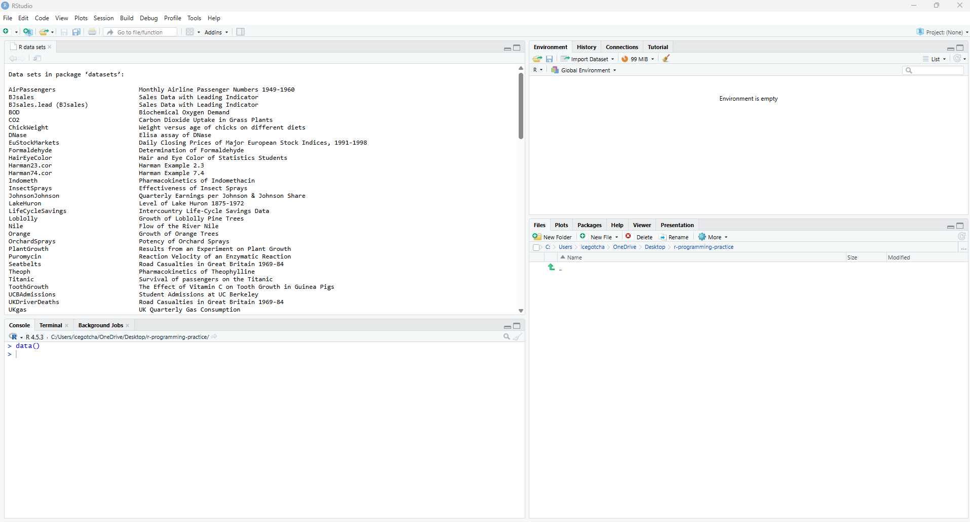
ในที่นี้เราจะใช้ USArrests
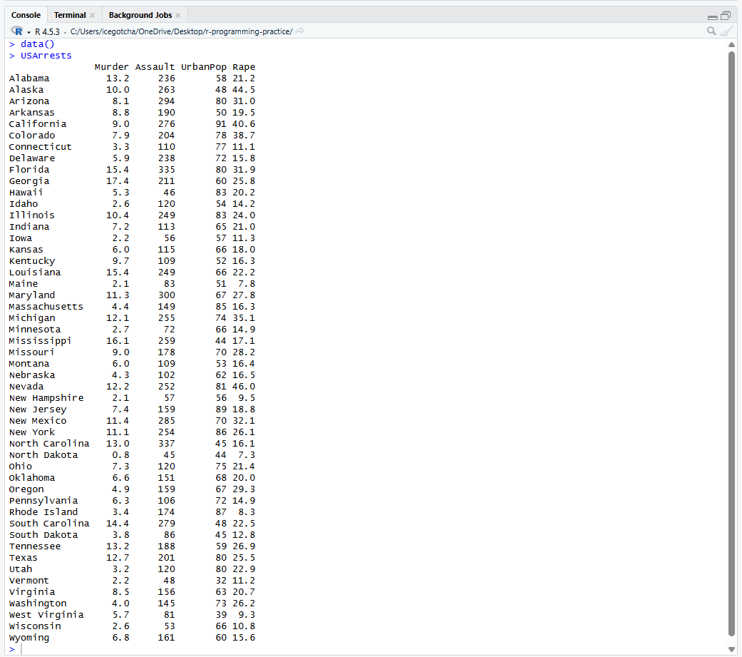
เราจะทำงานกับ Data Set นี้กัน
> class(USArrests)
[1] "data.frame"
> View(USArrests)
> ## Find mean of every column
> mean(USArrests$Murder)
[1] 7.788
> mean(USArrests$Assault)
[1] 170.76
> mean(USArrests$UrbanPop)
[1] 65.54
> mean(USArrests$Rape)
[1] 21.232
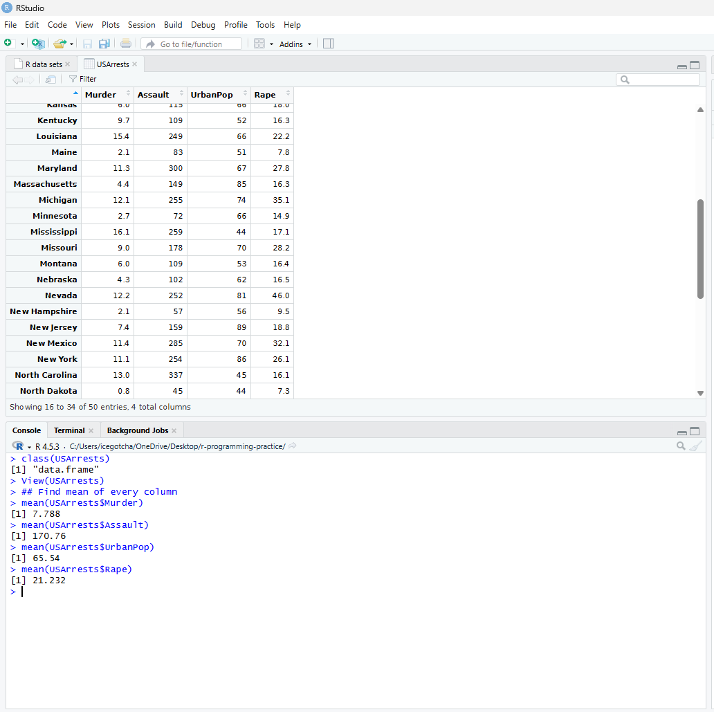
หากต้องการหา Mean ของทุกคอลัมน์ เราจะไม่รันคำสั่งเรียง ๆ กันอย่างนี้แน่ ๆ
ในการเขียนโปรแกรม เราจะมีหลักการที่เรียกว่า DRY (Don't Repeat Yourself) เราจะเขียนคำสั่งต่าง ๆ ในครั้งเดียวเท่านั้น
คำสั่งที่เราใช้ได้
## จำนวนแถว
> nrow(USArrests)

## จำนวนคอลัมน์
> ncol(USArrests)

## Preview table first 6 rows
> head(USArrests)
เราจะเขียนลูป for เพื่อหา mean ของทุกคอลัมน์
cal_mean_by_col <- function(df) {
	for (i in 1:ncol(df)) {
		name_col <- names(df)[i]
		mean_col <- mean(dfi)
		print(paste(name_col, ":", mean_col))
	}
}
ผลลัพธ์
> cal_mean_by_col(USArrests)
[1] "Murder : 7.788"
[1] "Assault : 170.76"
[1] "UrbanPop : 65.54"
[1] "Rape : 21.232"
apply()
เราสามารถใช้ฟังก์ชันนี้แทนการเขียน for loop
apply(USArrests, MARGIN=2, mean)

## Result

 Murder  Assault UrbanPop     Rape
   7.788  170.760   65.540   21.232
Note: ถ้าต้องการให้ลูปจำนวนแถวแทน กำหนด MARGIN=1
Documentation: https://www.rdocumentation.org/packages/base/versions/3.6.2/topics/apply
Working with Data
R สามารถอ่านข้อมูลได้หลายรูปแบบ
.txt.csv.xlsx.json.db(sqlite database)- Google Sheets
- SQL databases เช่น PostgreSQL, MySQL, MS SQL, BigQuery, AWS RedShift
แต่ต้องติดตั้งและ Include Library เพิ่ม
# install packages
install.packages(c("readr",
    "readxl",
    "googlesheets4",
    "jsonlite",
    "dplyr",
    "sqldf",
    "RSQLite"))

# load library
library(readr)
library(readxl)
library(googlesheets4)
library(jsonlite)
library(dplyr)
library(sqldf)
library(RSQLite)
Note:
install.packages ทำงานทีหนึ่งต้อง Restart R Server ทำงานครั้งเดียวก็สามารถโหลด library ใช้ไนโปรแกรมได้หลายครั้งเลย ไม่จำเป็นต้องทำคำสั่งซ้ำ
เราสามารถติดตั้ง Library ผ่าน R Studio ในแท็บ Packages
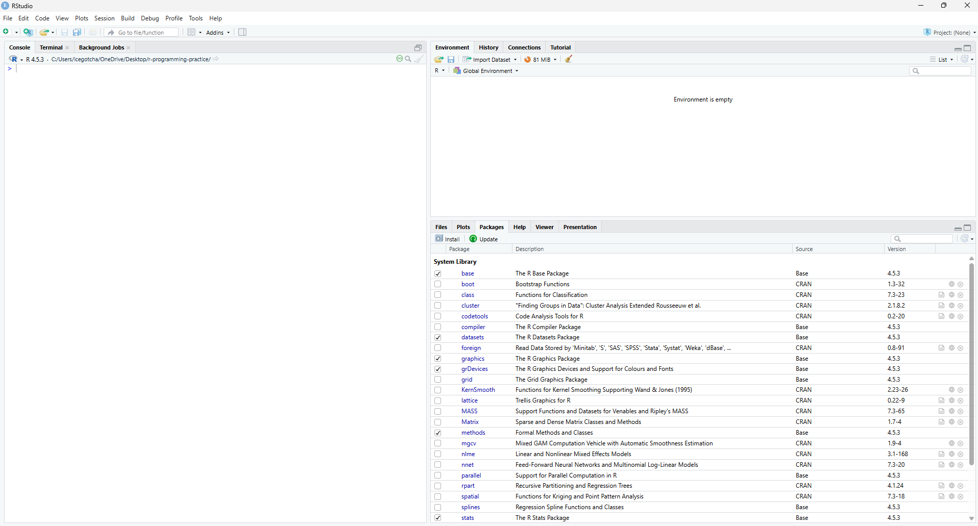
ดู Packages เต็ม ๆ ได้ที่ https://cran.r-project.org/web/packages/available_packages_by_name.html
Read text file
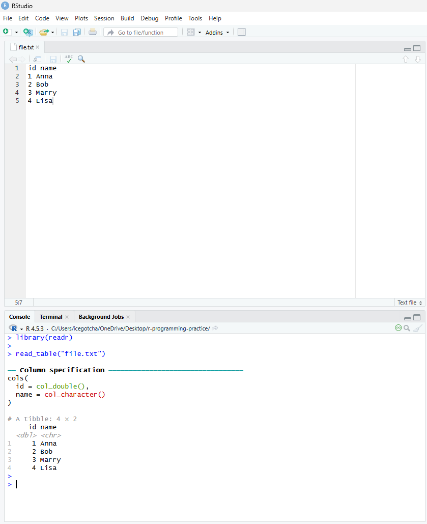
เรามี text file ลักษณะเป็นแบบนี้
id name
1 Anna
2 Bob
3 Marry
4 Lisa
เราจะอ่านไฟล์แบบนี้
โหลด Library readr
library(readr)
วิธีการอ่าน
people <- read_table("file.txt")
View(people)
เราจะได้ Data Frame พร้อมใช้งาน
Read CSV file
CSV โดยทั่วไปจะมีลักษณะเป็นอย่างนี้
id,name
1,Anna
2,Bob
3,Marry
4,Lisa
ใช้ Library เดียวกันคือ readr
เราจะอ่านไฟล์แบบนี้
people <- read_csv("file.csv")
Read Excel file
ตัวอย่างไฟล์
library(readxl)

## อ่านข้อมูลใน Sheet ที่ 1
people <- read_excel("students.xlsx", sheet=1)

## ใส่เป็นชื่อก็ได้
people <- read_excel("students.xlsx", sheet="Economics")
เก็บทุก Sheet ใน List
result <- list()

for (i in 1:3) {
	resulti <- read_excel("students.xlsx", sheet=i)
}

result1
result2
result3
Google Sheet
เราต้อง Share as link
แล้วโหลด library googlesheet4
library(googlesheet4)
ถ้าเป็น Public (คือไม่ต้อง login ก่อนเข้าไปดู) ให้เราเรียกคำสั่ง gs4_deauth() ก่อน เพื่อให้ข้ามการ authentation ไป
url ที่ใช้ เราจะตัด /edit?usp=sharing หรืออะไรตามหลัง ID ข้างหลัง /d/ ออก
url <- "..."
sheet_name <- "..."

gs4_deauth()

read_sheet(url, sheet=sheet_name)
การนำเอาตารางมารวมกัน
เรามีข้อมูลจากหลายที่ ถ้าต้องการรวมกันเป็นก้อนเดียว เช่น เรามีตารางจากหลาย sheet ต้องการเอามารวมเป็นตารางเดียว เราทำได้โดยการใช้คำสั่ง bind_rows()
โหลด library ก่อน
library(dplyr)
bind_rows(df1, df2, df3)

## create from list
df_list <- list(df1, df2, df3)
full_df <- bind_rows(df_list)
การทำงานของฟังก์ชันนี้เท่ากับ UNION ALL ใน SQL
ต่อคอลัมน์
เราใช้ bind_cols() ได้ แต่ข้อควรระวัง คือ ฟังก์ชันนี้จะใช้การต่อตรง ๆ ไม่ได้ดูการเชื่อมโยงของข้อมูล ก่อนใช้ควรให้แน่ใจว่าแต่ละแถวตรงกันหรือยัง
bind_cols(df1, df2)
ถ้าต้องการใช้ join จริง ๆ ต้องเปลี่ยนเป็นฟังก์ชัน
inner_joinleft_joinright_joinfull_joinanti_joinsemi_join- cross join (ด้วยฟังก์ชัน
tidyr::crossing())
ตัวอย่าง
left_join(d1, d2, by="id")
การใช้คำสั่ง SQL กับ Data frame
เราสามารถเล่นคำสั่ง SQL เพื่อจัดการข้อมูลได้ ไม่นับว่าข้อมูลจะต้องมาจาก Database จริง ต่อให้มาจาก txt ไฟล์ ถ้ามาอยู่ในรูปแบบ Data Frame ก็ทำได้
library(sqldf)

// read data

school <- read_csv("school.csv")

school_result <- sqldf("select * from school;")

school_avg_sum <- sqldf("select avg(student), sum(student) from school;")

usa_school <- sqldf("select * from school where country = 'USA';")
อ่านข้อมูลจาก SQLite
# load library
library(RSQLite)

# connect to SQLite database(.db file)
# 1. open connection
conn < -dbConnect(SQLite(), "chinook.db")

# 2. get data
dbListTables(conn)
dbListFields(conn, "customers")

df < -dbGetQuery(conn, "select * from customers where country = 'USA'")

# 3. close connection
dbDisconnect(conn)
บันทึกข้อมูลและ Environment ใน R
เราสามารถเซฟทุกอย่างที่ทำงานมาในรูปแบบไฟล์ .RData โดยใช้คำสั่ง save.images()
save.images(file="data.RData")
ถ้าจะโหลดมาใช้ก็ใช้คำสั่ง load()
load(file="data.RData")
ถ้าต้องการเก็บแค่ก้อนเดียว สามารถนำ Variables เข้าฟังก์ชัน saveRDS()
saveRDS(df, file="df_result.rds")
ถ้าจะโหลดก็
loadRDS("df_result.rds")
จบ